# Appendix: Stochastic direct and indirect effects {#stochastic}
```{r}
#| label: load-renv
#| echo: false
#| message: false
renv::autoload()
library(here)
```
## Definition of the effects
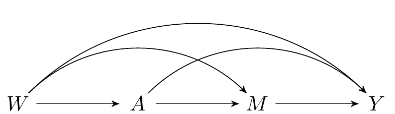
Consider the following directed acyclic graph.
```{tikz}
#| fig-cap: Directed acyclic graph under no intermediate confounders of the mediator-outcome relation affected by treatment
\dimendef\prevdepth=0
\pgfdeclarelayer{background}
\pgfsetlayers{background,main}
\usetikzlibrary{arrows,positioning}
\tikzset{
>=stealth',
punkt/.style={
rectangle,
rounded corners,
draw=black, very thick,
text width=6.5em,
minimum height=2em,
text centered},
pil/.style={
->,
thick,
shorten <=2pt,
shorten >=2pt,}
}
\newcommand{\Vertex}[2]
{\node[minimum width=0.6cm,inner sep=0.05cm] (#2) at (#1) {$#2$};
}
\newcommand{\VertexR}[2]
{\node[rectangle, draw, minimum width=0.6cm,inner sep=0.05cm] (#2) at (#1) {$#2$};
}
\newcommand{\ArrowR}[3]
{ \begin{pgfonlayer}{background}
\draw[->,#3] (#1) to[bend right=30] (#2);
\end{pgfonlayer}
}
\newcommand{\ArrowL}[3]
{ \begin{pgfonlayer}{background}
\draw[->,#3] (#1) to[bend left=45] (#2);
\end{pgfonlayer}
}
\newcommand{\EdgeL}[3]
{ \begin{pgfonlayer}{background}
\draw[dashed,#3] (#1) to[bend right=-45] (#2);
\end{pgfonlayer}
}
\newcommand{\Arrow}[3]
{ \begin{pgfonlayer}{background}
\draw[->,#3] (#1) -- +(#2);
\end{pgfonlayer}
}
\begin{tikzpicture}
  \Vertex{-4, 0}{W}
  \Vertex{0, 0}{M}
  \Vertex{-2, 0}{A}
  \Vertex{2, 0}{Y}
  \Arrow{W}{A}{black}
  \Arrow{A}{M}{black}
  \Arrow{M}{Y}{black}
  \ArrowL{W}{Y}{black}
  \ArrowL{A}{Y}{black}
  \ArrowL{W}{M}{black}
\end{tikzpicture}
```
## Motivation for stochastic interventions
- So far we have discussed controlled, natural, and interventional (in)direct
effects
- These effects require that $0 < \P(A=1\mid W) < 1$
- They are defined only for binary exposures
- _What can we do when the positivity assumption does not hold or the exposure
is continuous?_
- Solution: We can use stochastic effects
## Definition of stochastic effects
There are two possible ways of defining stochastic effects:
- Consider the effect of an intervention where the exposure is drawn from a
distribution
- For example incremental propensity score interventions
- Consider the effect of an intervention where the post-intervention exposure is
a function of the actually received exposure
- For example modified treatment policies
- In both cases $A \mid W$ is a non-deterministic intervention, thus the name
_stochastic intervention_
### Example: incremental propensity score interventions (IPSI) [@kennedy2018nonparametric] {#ipsi}
#### Definition of the intervention {.unnumbered}
- Assume $A$ is binary, and $\P(A=1\mid W=w) = g(1\mid w)$ is the propensity score
- Consider an intervention in which each individual receives the intervention
with probability $g_\delta(1\mid w)$, equal to
\begin{equation*}
g_\delta(1\mid w)=\frac{\delta g(1\mid w)}{\delta g(1\mid w) +
1 - g(1\mid w)}
\end{equation*}
- e.g., draw the post-intervention exposure from a Bernoulli variable with
probability $g_\delta(1\mid w)$
- The value $\delta$ is user given
- Let $A_\delta$ denote the post-intervention exposure distribution
- Some algebra shows that $\delta$ is an odds ratio comparing the pre- and
post-intervention exposure distributions
\begin{equation*}
\delta = \frac{\text{odds}(A_\delta = 1\mid W=w)}
{\text{odds}(A = 1\mid W=w)}
\end{equation*}
- Interpretation: _what would happen in a
world where the odds of receiving treatment is increased by $\delta$_
- Let $Y_{A_\delta}$ denote the outcome in this hypothetical world
#### Illustrative application for IPSIs
- Consider the effect of participation in sports on children's BMI
- Mediation through snacking, exercising, etc.
- Intervention: for each individual, increase the odds of participating in
sports by $\delta=2$
- The post-intervention exposure is a draw $A_\delta$ from a Bernoulli
distribution with probability $g_\delta(1\mid w)$
### Example: modified treatment policies (MTP) [@diaz2020causal] {.unnumbered}
#### Definition of the intervention {.unnumbered}
- Consider a continuous exposure $A$ taking values in the real numbers
- Consider an intervention that assigns exposure as $A_\delta = A - \delta$
- Example: $A$ is pollution measured as $PM_{2.5}$ and you are interested in an
intervention that reduces $PM_{2.5}$ concentration by some amount $\delta$
### Mediation analysis for stochastic interventions
- The total effect of an IPSI can be computed as a contrast of the outcome under
intervention vs no intervention:
\begin{equation*}
\psi = \E[Y_{A_\delta} - Y]
\end{equation*}
- Recall the NPSEM
\begin{align*}
W & = f_W(U_W)\\
A & = f_A(W, U_A)\\
M & = f_M(W, A, U_M)\\
Y & = f_Y(W, A, M, U_Y)
\end{align*}
- From this we have
\begin{align*}
M_{A_\delta} & = f_M(W, A_\delta, U_M)\\
Y_{A_\delta} & = f_Y(W, A_\delta, M_{A_\delta}, U_Y)
\end{align*}
- Thus, we have $Y_{A_\delta} = Y_{A_\delta, M_{A_\delta}}$ and $Y =
Y_{A,M_{A}}$
- Let us introduce the counterfactual $Y_{A_\delta, M}$, interpreted as the
outcome observed in a world where the intervention on $A$ is performed but the
mediator is fixed at the value it would have taken under no intervention:
\[Y_{A_\delta, M} = f_Y(W, A_\delta, M, U_Y)\]
- Then we can decompose the total effect into:
\begin{align*}
\E[Y&_{A_\delta,M_{A_\delta}} - Y_{A,M_A}] = \\
&\underbrace{\E[Y_{\color{red}{A_\delta},\color{blue}{M_{A_\delta}}} -
Y_{\color{red}{A_\delta},\color{blue}{M}}]}_{\text{stochastic natural
indirect effect}} +
\underbrace{\E[Y_{\color{blue}{A_\delta},\color{red}{M}} -
Y_{\color{blue}{A},\color{red}{M}}]}_{\text{stochastic natural direct
effect}}
\end{align*}
## Identification assumptions
- Confounder assumptions:
+ $A \indep Y_{a,m} \mid W$
+ $M \indep Y_{a,m} \mid W, A$
- No confounder of $M\rightarrow Y$ affected by $A$
- Positivity assumptions:
+ If $g_\delta(a \mid w)>0$ then $g(a \mid w)>0$
+ If $\P(M=m\mid W=w)>0$ then $\P(M=m\mid A=a,W=w)>0$
Under these assumptions, stochastic effects are identified as follows
- The indirect effect can be identified as follows
\begin{align*}
\E&(Y_{A_\delta} - Y_{A_\delta, M}) =\\
&\E\left[\color{Goldenrod}{\sum_{a}\color{ForestGreen}{\{\E(Y\mid A=a, W)
-\E(Y\mid A=a, M, W)\}}g_\delta(a\mid W)}\right]
\end{align*}
- The direct effect can be identified as follows
\begin{align*}
\E&(Y_{A_\delta} - Y_{A_\delta, M}) =\\
&\E\left[\color{Goldenrod}{\sum_{a}\color{ForestGreen}{\{\E(Y\mid A=a, M, W)
- Y\}}g_\delta(a\mid W)}\right]
\end{align*}
- Let's dissect the formula for the indirect effect in R:
```{r}
n <- 1e6
w <- rnorm(n)
a <- rbinom(n, 1, plogis(1 + w))
m <- rnorm(n, w + a)
y <- rnorm(n, w + a + m)
```
- First, fit regressions of the outcome on $(A,W)$ and $(M,A,W)$:
```{r}
fit_y1 <- lm(y ~ m + a + w)
fit_y2 <- lm(y ~ a + w)
```
- Get predictions fixing $A=a$ for all possible values $a$
```{r}
pred_y1_a1 <- predict(fit_y1, newdata = data.frame(a = 1, m, w))
pred_y1_a0 <- predict(fit_y1, newdata = data.frame(a = 0, m, w))
pred_y2_a1 <- predict(fit_y2, newdata = data.frame(a = 1, w))
pred_y2_a0 <- predict(fit_y2, newdata = data.frame(a = 0, w))
```
- Compute \[\color{ForestGreen}{\{\E(Y\mid A=a, W)-\E(Y\mid A=a, M, W)\}}\] for
each value $a$
```{r}
pseudo_a1 <- pred_y2_a1 - pred_y1_a1
pseudo_a0 <- pred_y2_a0 - pred_y1_a0
```
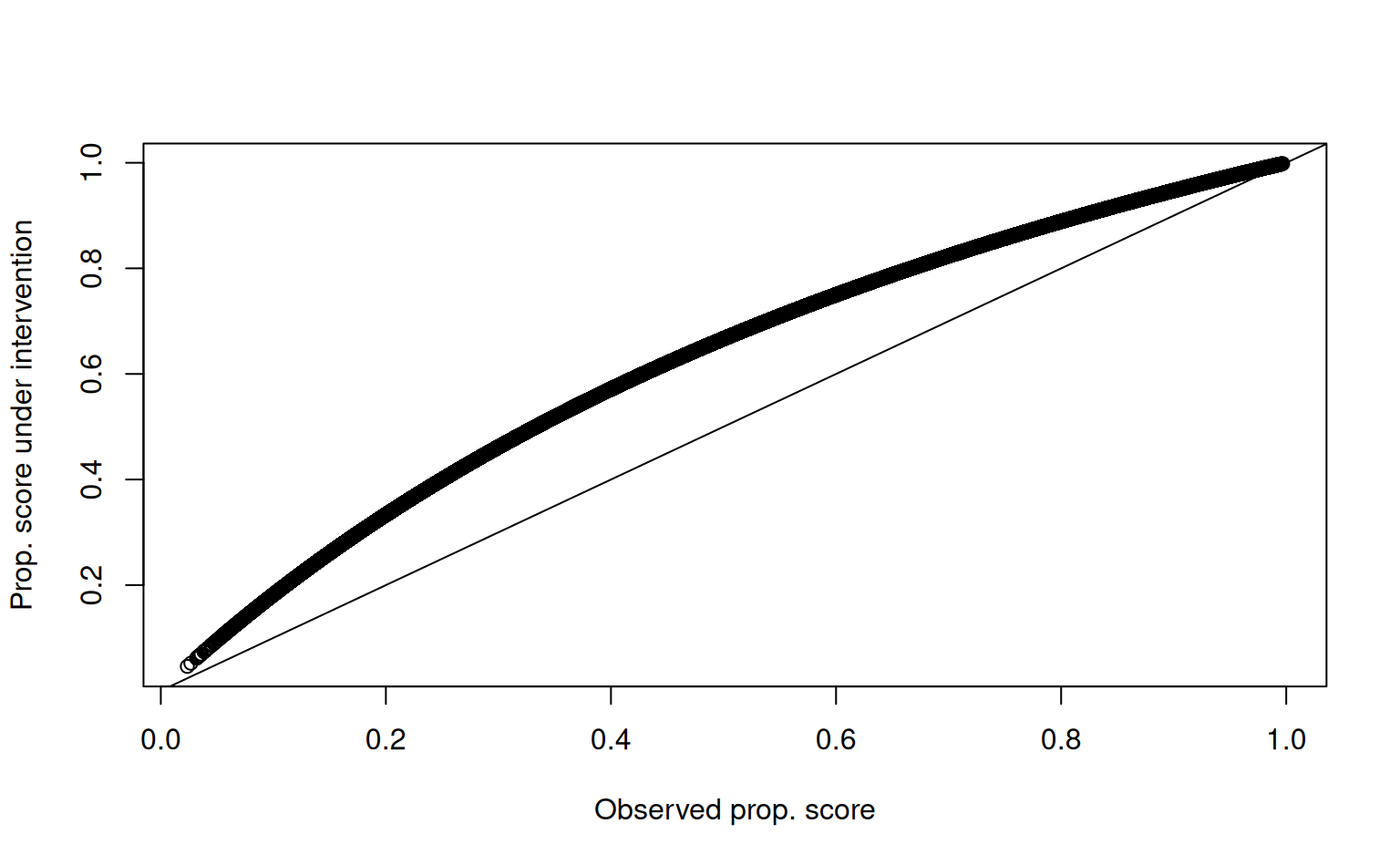
- Estimate the propensity score $g(1\mid w)$ and evaluate the post-intervention
propensity score $g_\delta(1\mid w)$
```{r}
pscore_fit <- glm(a ~ w, family = binomial())
pscore <- predict(pscore_fit, type = "response")
## How do the intervention vs observed propensity score compare
pscore_delta <- 2 * pscore / (2 * pscore + 1 - pscore)
```
- What do the post-intervention propensity scores look like?
```{r}
plot(pscore, pscore_delta,
xlab = "Observed prop. score",
ylab = "Prop. score under intervention"
)
abline(0, 1)
```
## What are the odds of exposure under intervention vs real world?
```{r}
odds <- (pscore_delta / (1 - pscore_delta)) / (pscore / (1 - pscore))
summary(odds)
```
- Compute the sum
\begin{equation*}
\color{Goldenrod}{\sum_{a}\color{ForestGreen}{\{\E(Y\mid A=a, W) -
\E(Y\mid A=a, M, W)\}}g_\delta(a\mid W)}
\end{equation*}
```{r}
indirect <- pseudo_a1 * pscore_delta + pseudo_a0 * (1 - pscore_delta)
```
- The average of this value is the indirect effect
```{r}
## E[Y(Adelta) - Y(Adelta, M)]
mean(indirect)
```
- The direct effect is
\begin{align*}
\E&(Y_{A_\delta} - Y_{A_\delta, M}) =\\
&\E\left[\color{Goldenrod}{\sum_{a}\color{ForestGreen}{\{\E(Y\mid A=a, M,
W) - Y\}}g_\delta(a\mid W)}\right]
\end{align*}
- Which can be computed as
```{r}
direct <- (pred_y1_a1 - y) * pscore_delta +
(pred_y1_a0 - y) * (1 - pscore_delta)
mean(direct)
```
## Summary
- Stochastic (in)direct effects
- Relax the positivity assumption
- Can be defined for non-binary exposures
- Do not require a cross-world assumption
- Still require the absence of intermediate confounders
- But, compared to the NDE and NIE, we can design a randomized study where
identifiability assumptions hold, at least in principle
- There is a version of these effects that can accommodate intermediate
confounders [@hejazi2020nonparametric]
- `R` implementation to be released soon...stay tuned!