# Types of path-specific causal mediation effects {#estimands}
```{r}
#| label: load-renv
#| echo: false
#| message: false
renv::autoload()
library(here)
```
- Controlled direct effects
- Natural direct and indirect effects
- Randomized interventional direct and indirect effects
- Path-specific effects using *recanting twins*
```{tikz}
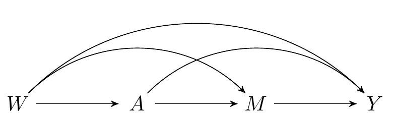
#| fig-cap: Directed acyclic graph under *no intermediate confounders* of the mediator-outcome relation affected by treatment
\dimendef\prevdepth=0
\pgfdeclarelayer{background}
\pgfsetlayers{background,main}
\usetikzlibrary{arrows,positioning}
\tikzset{
>=stealth',
punkt/.style={
rectangle,
rounded corners,
draw=black, very thick,
text width=6.5em,
minimum height=2em,
text centered},
pil/.style={
->,
thick,
shorten <=2pt,
shorten >=2pt,}
}
\newcommand{\Vertex}[2]
{\node[minimum width=0.6cm,inner sep=0.05cm] (#2) at (#1) {$#2$};
}
\newcommand{\VertexR}[2]
{\node[rectangle, draw, minimum width=0.6cm,inner sep=0.05cm] (#2) at (#1) {$#2$};
}
\newcommand{\ArrowR}[3]
{ \begin{pgfonlayer}{background}
\draw[->,#3] (#1) to[bend right=30] (#2);
\end{pgfonlayer}
}
\newcommand{\ArrowL}[3]
{ \begin{pgfonlayer}{background}
\draw[->,#3] (#1) to[bend left=45] (#2);
\end{pgfonlayer}
}
\newcommand{\EdgeL}[3]
{ \begin{pgfonlayer}{background}
\draw[dashed,#3] (#1) to[bend right=-45] (#2);
\end{pgfonlayer}
}
\newcommand{\Arrow}[3]
{ \begin{pgfonlayer}{background}
\draw[->,#3] (#1) -- +(#2);
\end{pgfonlayer}
}
\begin{tikzpicture}
  \Vertex{-4, 0}{W}
  \Vertex{0, 0}{M}
  \Vertex{-2, 0}{A}
  \Vertex{2, 0}{Y}
  \Arrow{W}{A}{black}
  \Arrow{A}{M}{black}
  \Arrow{M}{Y}{black}
  \ArrowL{W}{Y}{black}
  \ArrowL{A}{Y}{black}
  \ArrowL{W}{M}{black}
\end{tikzpicture}
```
## Controlled direct effects
$$\psi_{\text{CDE}} = \E(Y_{1,m} - Y_{0,m})$$
{width="40%"}
- Intervening on the SCM to set $M=m$ uniformly for everyone in the population
- Compare $A=1$ vs $A=0$ with $M=m$ fixed
### Identification assumptions:
- Confounder assumptions:
- $A \indep Y_{a,m} \mid W$
- $M \indep Y_{a,m} \mid W, A$
- Positivity assumptions:
- $\P(M = m \mid A=a, W) > 0 \text{ } a.e.$
- $\P(A=a \mid W) > 0 \text{ } a.e.$
Under the above identification assumptions, the controlled direct effect can be identified: $$
\E(Y_{1,m} - Y_{0,m}) = \E\{ \color{ForestGreen}{\E(Y \mid A=1, M=m, W) -
\E(Y \mid A=0, M=m, W)} \}
$$
- For intuition about this formula in R, let's continue with a toy example:
```{webr-r}
n <- 1e6
w <- rnorm(n)
a <- rbinom(n, 1, 0.5)
m <- rnorm(n, w + a)
y <- rnorm(n, w + a + m)
```
- First we fit a correct model for the outcome
```{webr-r}
lm_y <- lm(y ~ m + a + w)
```
- Assume we would like the CDE at $m=0$
- Then we generate predictions $$
\color{ForestGreen}{\E(Y \mid A=1, M=m, W)}
\text{ and } \color{ForestGreen}{\E(Y \mid A=0, M=m, W)} \ :
$$
```{webr-r}
pred_y1 <- predict(lm_y, newdata = data.frame(a = 1, m = 0, w = w))
pred_y0 <- predict(lm_y, newdata = data.frame(a = 0, m = 0, w = w))
```
- Then we compute the difference between the predicted values $\color{ForestGreen}{\E(Y \mid A=1, M=m, W) - \E(Y \mid A=0, M=m, W)}$, and average across values of $W$
```{webr-r}
## CDE at m = 0
mean(pred_y1 - pred_y0)
```
### Is this the estimand I want?
- Makes the most sense if it is reasonable for everyone have a constant level $m
\in \mathcal{M}$.
- Judea Pearl calls this *prescriptive*.
- Can you think of an example? (Air pollution, rescue inhaler dosage, hospital visits...)
- Does not provide a decomposition of the average treatment effect into direct and indirect effects.
*What if everyone having the same value of the mediator doesn't make sense?*
*What if we want to decompose the average treatment effect into its direct and indirect counterparts?*
## Natural direct and indirect effects
Continuing to use the same DAG as above,
- Recall the definition of the nested counterfactual: \begin{equation*}
Y_{1, M_0} = f_Y(W, 1, M_0, U_Y)
\end{equation*}
- Interpreted as *the outcome for an individual in a hypothetical world where treatment was given but the mediator was held at the value it would have taken under no treatment*
{width="40%"}
- Recall that, because of the definition of counterfactuals \begin{equation*}
Y_{1, M_1} = Y_1
\end{equation*}
Then we can decompose the *average treatment effect* $\E(Y_1-Y_0)$ as follows
\begin{equation*}
\E[Y_{1,M_1} - Y_{0,M_0}] = \underbrace{\E[Y_{\color{red}{1},\color{blue}{M_1}}
- Y_{\color{red}{1},\color{blue}{M_0}}]}_{\text{natural indirect effect}} +
\underbrace{\E[Y_{\color{blue}{1},\color{red}{M_0}} -
Y_{\color{blue}{0},\color{red}{M_0}}]}_{\text{natural direct effect}}
\end{equation*}
- Natural direct effect (NDE): Varying treatment while keeping the mediator fixed at the value it would have taken under no treatment
- Natural indirect effect (NIE): Varying the mediator from the value it would have taken under treatment to the value it would have taken under control, while keeping treatment fixed
### Identification assumptions:
- $A \indep Y_{a,m} \mid W$
- $M \indep Y_{a,m} \mid W, A$
- $A \indep M_a \mid W$
- $M_0 \indep Y_{1,m} \mid W$
- and positivity assumptions
### Cross-world independence assumption
What does $M_0 \indep Y_{1,m} \mid W$ mean?
- Conditional on $W$, knowledge of the mediator value in the absence of treatment, $M_0$, provides no information about the outcome under treatment, $Y_{1,m}$.
- Can you think of a data-generating mechanism that would violate this assumption?
- Example: in a randomized study, whenever we believe that treatment assignment works through adherence (i.e., almost always), we are violating this assumption (more on this later).
- Cross-world assumptions are problematic for other reasons, including:
- You can never design a randomized study where the assumption holds by design.
**If the cross-world assumption holds, can write the NDE as a weighted average of controlled direct effects at each level of** $M=m$.
$$
\E \sum_m \{\E(Y_{1,m} \mid W) - \E(Y_{0,m} \mid W)\} \P(M_{0}=m \mid W)
$$
- If CDE($m$) is constant across $m$, then CDE = NDE.
### Identification formula:
- Under the above identification assumptions, the natural direct effect can be identified: \begin{equation*}
\E(Y_{1,M_0} - Y_{0,M_0}) =
\E[\color{red}{\E\{}\color{ForestGreen}{\E(Y \mid A=1, M, W) -
\E(Y \mid A=0, M, W)}\color{red}{\mid A=0,W\}}]
\end{equation*}
- The natural indirect effect can be identified similarly.
- Let's dissect this formula in `R`:
```{webr-r}
n <- 1e6
w <- rnorm(n)
a <- rbinom(n, 1, 0.5)
m <- rnorm(n, w + a)
y <- rnorm(n, w + a + m)
```
- First we fit a correct model for the outcome
```{webr-r}
lm_y <- lm(y ~ m + a + w)
```
- Then we generate predictions $\color{ForestGreen}{\E(Y \mid A=1, M, W)}
\text{ and }\color{ForestGreen}{\E(Y \mid A=0, M, W)}$ with $A$ fixed but letting $M$ and $W$ take their observed values
```{webr-r}
pred_y1 <- predict(lm_y, newdata = data.frame(a = 1, m = m, w = w))
pred_y0 <- predict(lm_y, newdata = data.frame(a = 0, m = m, w = w))
```
- Then we compute the difference between the predicted values $\color{ForestGreen}{\E(Y \mid A=1, M, W) - \E(Y \mid A=0, M, W)},$
- and use this difference as a pseudo-outcome in a regression on $A$ and $W$: $\color{red}{\E\{}\color{ForestGreen}{\E(Y \mid A=1, M, W) -
\E(Y \mid A=0, M, W)}\color{red}{\mid A=0,W\}}$
```{webr-r}
pseudo <- pred_y1 - pred_y0
lm_pseudo <- lm(pseudo ~ a + w)
```
- Now we predict the value of this pseudo-outcome under $A=0$, and average the result
```{webr-r}
pred_pseudo <- predict(lm_pseudo, newdata = data.frame(a = 0, w = w))
## NDE:
mean(pred_pseudo)
```
### Is this the estimand I want?
- Makes sense to hypothetically set $A$ but not $M$.
- Want to understand a natural mechanism underlying an association or total effect. Judea Pearl calls this *descriptive*.
- NDE + NIE = total effect (ATE).
- Okay with the assumptions.
*What if our data structure involves a post-treatment confounder of the mediator-outcome relationship (e.g., adherence)?*
```{tikz}
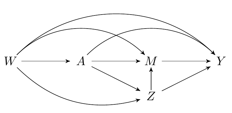
#| fig-cap: Directed acyclic graph under intermediate confounders of the mediator-outcome relation affected by treatment
\dimendef\prevdepth=0
\pgfdeclarelayer{background}
\pgfsetlayers{background,main}
\usetikzlibrary{arrows,positioning}
\tikzset{
>=stealth',
punkt/.style={
rectangle,
rounded corners,
draw=black, very thick,
text width=6.5em,
minimum height=2em,
text centered},
pil/.style={
->,
thick,
shorten <=2pt,
shorten >=2pt,}
}
\newcommand{\Vertex}[2]
{\node[minimum width=0.6cm,inner sep=0.05cm] (#2) at (#1) {$#2$};
}
\newcommand{\VertexR}[2]
{\node[rectangle, draw, minimum width=0.6cm,inner sep=0.05cm] (#2) at (#1) {$#2$};
}
\newcommand{\ArrowR}[3]
{ \begin{pgfonlayer}{background}
\draw[->,#3] (#1) to[bend right=30] (#2);
\end{pgfonlayer}
}
\newcommand{\ArrowL}[3]
{ \begin{pgfonlayer}{background}
\draw[->,#3] (#1) to[bend left=45] (#2);
\end{pgfonlayer}
}
\newcommand{\EdgeL}[3]
{ \begin{pgfonlayer}{background}
\draw[dashed,#3] (#1) to[bend right=-45] (#2);
\end{pgfonlayer}
}
\newcommand{\Arrow}[3]
{ \begin{pgfonlayer}{background}
\draw[->,#3] (#1) -- +(#2);
\end{pgfonlayer}
}
\begin{tikzpicture}
  \Vertex{0, -1}{Z}
  \Vertex{-4, 0}{W}
  \Vertex{0, 0}{M}
  \Vertex{-2, 0}{A}
  \Vertex{2, 0}{Y}
  \ArrowR{W}{Z}{black}
  \Arrow{Z}{M}{black}
  \Arrow{W}{A}{black}
  \Arrow{A}{M}{black}
  \Arrow{M}{Y}{black}
  \Arrow{A}{Z}{black}
  \Arrow{Z}{Y}{black}
  \ArrowL{W}{Y}{black}
  \ArrowL{A}{Y}{black}
  \ArrowL{W}{M}{black}
\end{tikzpicture}
```
{width="80%"}
### Unidentifiability of the NDE and NIE in this setting
- In this example, natural direct and indirect effects are not generally point identified from observed data $O=(W,A,Z,M,Y)$.
- The reason for this is that the cross-world counterfactual assumption $$Y_{1,m} \indep M_0 \mid W$$ does not hold in the above directed acyclic graph.
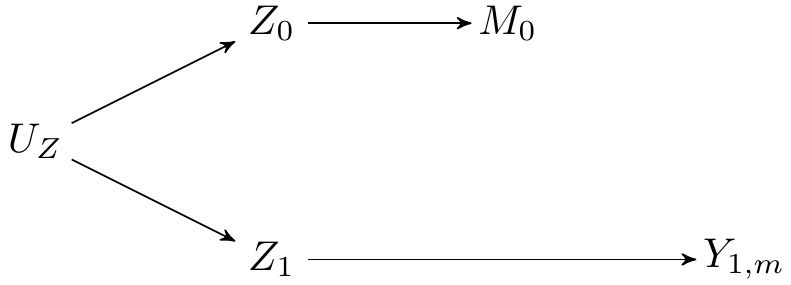
- To give intuition, we focus on the counterfactual outcome $Y_{A=1, M_{A=0}}$.
- This counterfactual outcome involves two counterfactual worlds simultaneously: one in which $A=1$ for the first portion of the counterfactual outcome, and one in which $A=0$ for the nested portion of the counterfactual outcome.
- Setting $A=1$ induces a counterfactual treatment-induced confounder, denoted $Z_{A=1}$. Setting $A=0$ induces another counterfactual treatment-induced confounder, denoted $Z_{A=0}$.
- The two treatment-induced counterfactual confounders, $Z_{A=1}$ and $Z_{A=0}$ share unmeasured common causes, $U_Z$, which creates a spurious association.
- Because $Z_{A=1}$ is causally related to $Y_{A=1, M=m}$, and $Z_{A=0}$ is also casually related to $M_{A=0}$, the path through $U_Z$ means that the backdoor criterion is not met for identification of $Y_{A=1, M_{A=0}}$, i.e., $M_{0} \notindep Y_{A=1, m} \mid W$, where $W$ denotes baseline covariates.
```{tikz}
#| fig-cap: Parallel worlds model of the scenario considered
\dimendef\prevdepth=0
\pgfdeclarelayer{background}
\pgfsetlayers{background,main}
\usetikzlibrary{arrows,positioning}
\tikzset{
>=stealth',
punkt/.style={
rectangle,
rounded corners,
draw=black, very thick,
text width=6.5em,
minimum height=2em,
text centered},
pil/.style={
->,
thick,
shorten <=2pt,
shorten >=2pt,}
}
\newcommand{\Vertex}[2]
{\node[minimum width=0.6cm,inner sep=0.05cm] (#2) at (#1) {$#2$};
}
\newcommand{\VertexR}[2]
{\node[rectangle, draw, minimum width=0.6cm,inner sep=0.05cm] (#2) at (#1) {$#2$};
}
\newcommand{\ArrowR}[3]
{ \begin{pgfonlayer}{background}
\draw[->,#3] (#1) to[bend right=30] (#2);
\end{pgfonlayer}
}
\newcommand{\ArrowL}[3]
{ \begin{pgfonlayer}{background}
\draw[->,#3] (#1) to[bend left=45] (#2);
\end{pgfonlayer}
}
\newcommand{\EdgeL}[3]
{ \begin{pgfonlayer}{background}
\draw[dashed,#3] (#1) to[bend left=45] (#2);
\end{pgfonlayer}
}
\newcommand{\EdgeR}[3]
{ \begin{pgfonlayer}{background}
\draw[dashed,#3] (#1) to[bend right=-45] (#2);
\end{pgfonlayer}
}
\newcommand{\Arrow}[3]
{ \begin{pgfonlayer}{background}
\draw[->,#3] (#1) -- +(#2);
\end{pgfonlayer}
}

\begin{tikzpicture}
  \Vertex{0, 1}{Z_0}
  \Vertex{0, -1}{Z_1}
  \Vertex{-2, 0}{U_Z}
  \Vertex{2, 1}{M_0}
  \Vertex{4, -1}{Y_{1, m}}
  \Arrow{Z_0}{M_0}{black}
  \Arrow{Z_1}{Y_{1, m}}{black}
  \Arrow{U_Z}{Z_0}{black}
  \Arrow{U_Z}{Z_1}{black}
\end{tikzpicture}
```
```{=html}
<!--
this is what we used to have
- Technically, the reason for this is that an intervention setting $A=1$
(necessary for the definition of $Y_{1,m}$) induces a counterfactual variable
$Z_1$.
- Likewise, an intervention setting $A=0$ (necessary for the definition of
$M_0$) induces a counterfactual $Z_0$.
- The variables $Z_1$ and $Z_0$ are correlated because they share unmeasured
common causes, $U_Z$.
- The variable $Z_1$ is correlated with $Y_{1,m}$, and the variable $Z_0$ is
correlated with $M_0$, because they are counterfactual outcomes in the same
hypothetical worlds.
- To see this in the definition of counterfactual from a causal structural
model:
\begin{align*}
Y_{1,m} &= f_Y(W, 1, Z_1, m, U_Y), \text{ and }\\
M_0 &= f_M(W, 0, Z_0, U_M)\\
\end{align*}
are correlated even after adjusting for $W$ by virtue of $Z_1$ and $Z_0$ being
correlated.
-->
```
```{=html}
<!--
Intuitively:
- $Z$ is a confounder of the relation $M \rightarrow Y$, which requires
adjustment
- But $Z$ is on the pathway $A\rightarrow Y$, which precludes adjustment
-->
```
However:
- We can actually identify the NIE/NDE if we are willing to invoke monotonicity between a treatment and one or more binary treatment-induced confounders [@tchetgen2014identification].
- Assuming monotonicity is also sometimes referred to as assuming "no defiers"---in other words, assuming that there are no individuals who would do the opposite of the encouragement.
- Monotonicity may seem like a restrictive assumption, but may be reasonable in some common scenarios (e.g., in trials where the intervention is randomized treatment assignment and the treatment-induced confounder is whether or not treatment was actually taken---in this setting, we may feel comfortable assuming that there are no "defiers", frequently assumed when using IVs to identify causal effects)
Note: CDEs are still identified in this setting. They can be identified and estimated similarly to a longitudinal data structure with a two-time-point intervention.
## Randomized interventional (in)direct effects
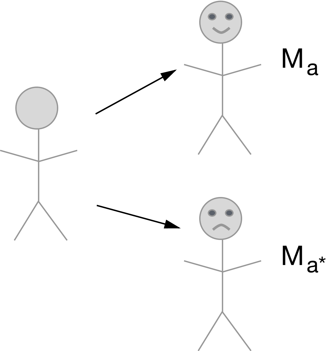
- Let $G_a$ denote a random draw from the distribution of $M_a \mid W$
- Define the counterfactual $Y_{1,G_0}$ as the counterfactual variable in a hypothetical world where $A$ is set $A=1$ and $M$ is set to $M=G_0$ with probability one.
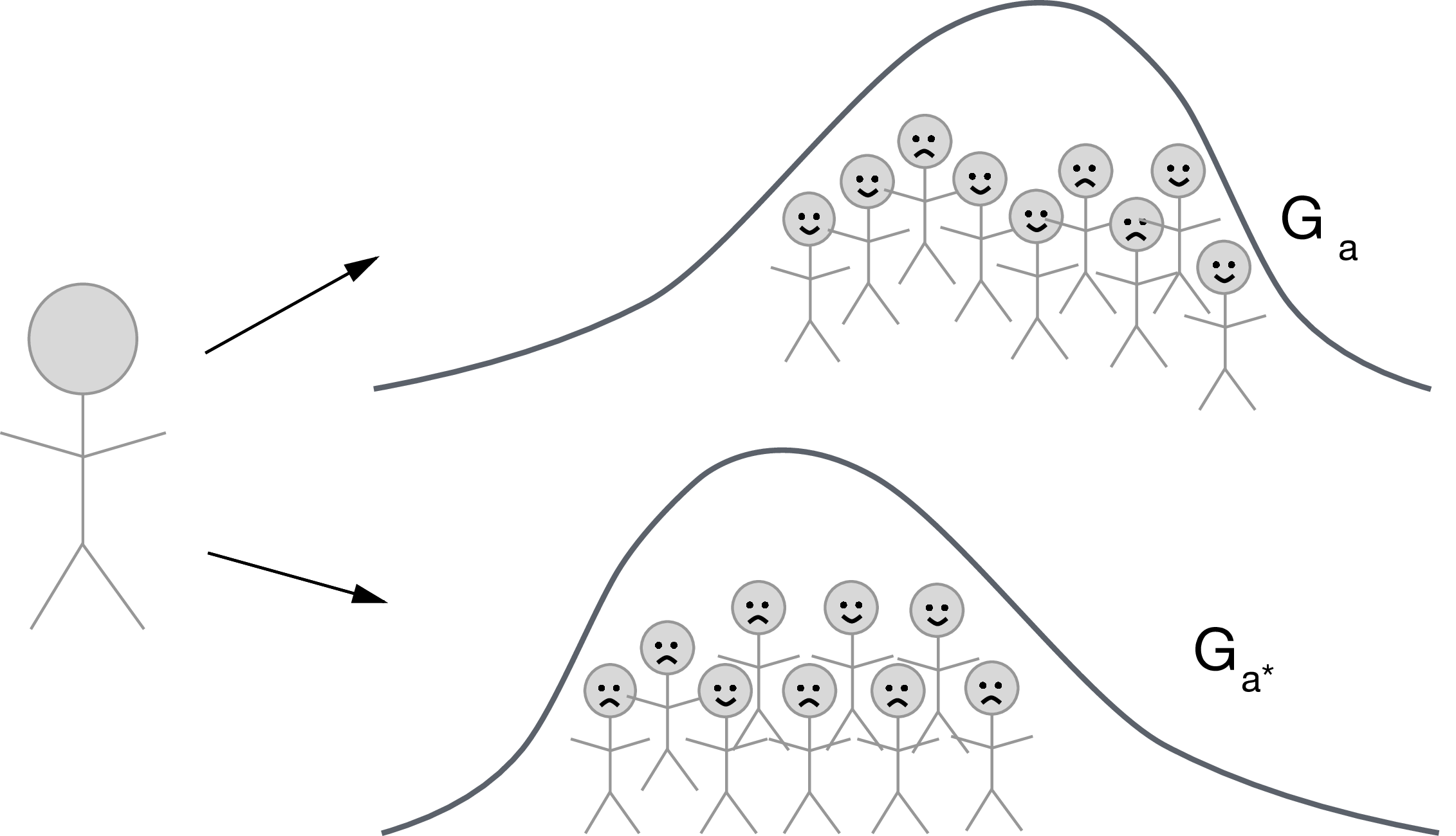{width="60%"}
- Define $Y_{0,G_0}$ and $Y_{1,G_1}$ similarly
- Then we can define: $$
\E[Y_{1,G_1} - Y_{0,G_0}] = \underbrace{\E[Y_{\color{red}{1},
\color{blue}{G_1}} - Y_{\color{red}{1},
\color{blue}{G_0}}]}_{\text{interventional indirect effect}} +
\underbrace{\E[Y_{\color{blue}{1},\color{red}{G_0}} -
Y_{\color{blue}{0},
\color{red}{G_0}}]}_{\text{interventional direct effect}}
$$
- Note that $\E[Y_{1,G_1} - Y_{0,G_0}]$ is still an *overall effect* of treatment, even if it is different from the ATE $\E[Y_{1} - Y_{0}]$
- We gain in the ability to solve a problem, but lose in terms of interpretation of the causal effect (cannot decompose the ATE)
### An alternative definition of the effects:
- Above we defined $G_a$ as a random draw from the distribution of $M_a \mid W$
- What if instead we define $G_a$ as a random draw from the distribution of $M_a \mid (Z_a,W)$
- It turns out the indirect effect defined in this way only measures the path $A \rightarrow M \rightarrow Y$, and not the path $A \rightarrow Z \rightarrow M \rightarrow Y$
- There may be important reasons to choose one over another (e.g., survival analyses where we want the distribution conditional on $Z$, instrumental variable designs where it doesn't make sense to condition on $Z$)
```{=html}
<!--
+ Marginal PIDE: $\E(Y_{a, g_{M \mid a^{\star}, W}}) -
\E(Y_{a^{\star}, g_{M \mid a^{\star}, W}})$
+ Marginal PIIE: $\E(Y_{a, g_{M \mid a, W}}) -
\E(Y_{a, g_{M \mid a^{\star}, W}})$
+ Conditional PIDE: $\E(Y_{a, g_{M \mid Z, a^{\star}, W}}) -
\E(Y_{a^{\star}, g_{M \mid Z, a^{\star}, W}})$
+ Conditional PIIE: $\E(Y_{a, g_{M \mid Z, a, W}}) -
\E(Y_{a, g_{M \mid Z, a^{\star}, W}})$
+ Can you think of an example when you would want the conditional versions?
Marginal versions?
-->
```
### Identification assumptions:
- $A \indep Y_{a,m} \mid W$
- $M \indep Y_{a,m} \mid W, A, Z$
- $A \indep M_a \mid W$
- and positivity assumptions.
Under these assumptions, the randomized interventional direct and indirect effect is identified: \begin{align*}
\E &(Y_{a, G_{a'}}) = \\
& \E\left[\color{Purple}{\E\left\{\color{red}{\sum_z}
\color{ForestGreen}{\E(Y \mid A=a, Z=z, M, W)}
\color{red}{\P(Z=z \mid A=a, W)}\mid A=a', W\right\}} \right]
\end{align*}
- Let's dissect this formula in `R`:
```{webr-r}
n <- 1e6
w <- rnorm(n)
a <- rbinom(n, 1, 0.5)
z <- rbinom(n, 1, 0.5 + 0.2 * a)
m <- rnorm(n, w + a - z)
y <- rnorm(n, w + a + z + m)
```
- Let us compute $\E(Y_{1, G_0})$ (so that $a = 1$, and $a'=0$).
- First, fit a regression model for the outcome, and compute $\color{ForestGreen}{\E(Y \mid A=a, Z=z, M, W)}$ for all values of $z$
```{webr-r}
lm_y <- lm(y ~ m + a + z + w)
pred_a1z0 <- predict(lm_y, newdata = data.frame(m = m, a = 1, z = 0, w = w))
pred_a1z1 <- predict(lm_y, newdata = data.frame(m = m, a = 1, z = 1, w = w))
```
- Now we fit the true model for $Z \mid A, W$ and get the conditional probability that $Z=1$ fixing $A=1$
```{webr-r}
prob_z <- lm(z ~ a)
pred_z <- predict(prob_z, newdata = data.frame(a = 1))
```
- Now we compute the following pseudo-outcome: $\color{red}{\sum_z}\color{ForestGreen}{\E(Y \mid A=a, Z=z, M, W)}
\color{red}{\P(Z=z \mid A=a, w)}$
```{webr-r}
pseudo_out <- pred_a1z0 * (1 - pred_z) + pred_a1z1 * pred_z
```
- Now we regress this pseudo-outcome on $A,W$, and compute the predictions setting $A=0$, that is, $$
\color{Purple}{\E\left\{\color{red}{\sum_z}
\color{ForestGreen}{\E(Y \mid A=a, Z=z, M, W)}
\color{red}{\P(Z=z \mid A=a, w)}\mid A=a', W\right\}}
$$
```{webr-r}
fit_pseudo <- lm(pseudo_out ~ a + w)
pred_pseudo <- predict(fit_pseudo, data.frame(a = 0, w = w))
```
- And finally, just average those predictions!
```{webr-r}
# Mean(Y(1, G(0)))
mean(pred_pseudo)
```
- This was for $(a,a')=(1,0)$. Can do the same with $(a,a')=(1,1)$, and $(a,a')=(0,0)$ to obtain an effect decomposition
\begin{equation*}
\E[Y_{1,G_1} - Y_{0,G_0}] = \underbrace{\E[Y_{\color{red}{1},
\color{blue}{G_1}} -
Y_{\color{red}{1},
\color{blue}{G_0}}]}_{\text{interventional indirect effect}} +
\underbrace{\E[Y_{\color{blue}{1},\color{red}{G_0}} -
Y_{\color{blue}{0},
\color{red}{G_0}}]}_{\text{interventional direct effect}}
\end{equation*}
### Is this the estimand I want?
- Do not want to intervene directly on $M$ in the causal model.
- Goal is to understand a descriptive type of mediation.
- Okay with the assumptions!
### But, there is an important limitation of randomized interventional effects
@miles2022causal recently uncovered an important limitation of these effects, which can be described as follows. The sharp mediational null hypothesis can be defined as
$$
H_0:Y(a, M(a')) = Y(a, M(a^\star));\text{ for all }a, a', a^\star \ .
$$
The problem is that randomized interventional effects are not guaranteed to be null when the sharp mediational hypothesis is true.
This could present a problem in practice if some subgroup of the population has a relationship between $A$ and $M$, but not between $M$ and $Y$. Then, another distinct subgroup of the population has a relationship between $M$ and $Y$ but not between $A$ and $M$. In such a scenario, the randomized interventional indirect effect would be nonzero, but there would be no one person in the population whose effect of $A$ on $Y$ would be mediated by $M$.
```{=html}
<!--
One counterexample involves creating an NPSEM with independent errors,
$W=\emptyset$, and an exogenous binary variable $U_Z$ such that $M(a)
= M(a')$ in the event $U_Z=1$ and $Y(a,m') = Y(a,m)$ in the event
$U_Z=0$ for all $a$, $a'$, and $m$, such that there is no causal
influence of $A$ on $Y$ operating through $M$. It is easy to see that
the randomized interventional indirect effect in this example equals
\[\sum_{z,m} E(Y\mid m, z,a) P(Z=z\mid a)[P(M=m\mid a)-P(M=m\mid
a')],\]
which is generally not null, and would only be null if $U_Z$
was observed and conditioned upon in all the above quantities.
-->
```
More details can be found in the original paper.
## Path-specific effects using *recanting twins*
The DAG we are working under contains four paths of interest:
\begin{align*}
P_1&: A\rightarrow Y;\\
P_2&: A \rightarrow Z \rightarrow Y;\\
P_3&: A \rightarrow Z \rightarrow M \rightarrow Y\\
P_4&: A \rightarrow M \rightarrow Y,
\end{align*}
Natural path-specific effects could be defined using the following nested counterfactuals: \begin{align*}
Y_{S_0}&=Y(1, Z(1), M(1, Z(1))),\\
Y_{S_1}&=Y(0, Z(1), M(1, Z(1))),\\
Y_{S_2}&=Y(0, Z(0), M(1, Z(1))),\\
Y_{S_3}&=Y(0, Z(0), M(1, Z(0))),\\
Y_{S_4}&=Y(0, Z(0), M(0, Z(0))),
\end{align*}
As before, the problem is that the distribution of $Y_{S_2}$ is not identifiable due to the so-called recanting witness $Z$. This means that one can contrast $Y_{S_1}$ with $Y_{S_3}$ but not with $Y_{S_2}$. Thus, the effects operating through $P_2$ and $P_3$ cannot be disentangled.
$Z$ is called a recanting witness because "it tells one story" $Z(1)$ for the purposes of one path, and another story $Z(0)$ for the purposes of the other.
But what if we replaced recanting witnesses by randomized versions of them that carry some of the same information? Specifically, if $T(a)$ is a random draw from the distribution of $Z(a)$ conditional on $W$, we can:
- Measure $P_2$ by contrasting $$
Y(0, Z(1), M(1, {\color{ForestGreen}{T(1)}})) \text{ vs. }
Y(0, Z(0), M(1, \color{ForestGreen}{T(1)}))
$$
- Measure $P_3$ by contrasting $$
Y(0, {\color{ForestGreen}{T(0)}}, M(1, Z(1))) \text{ vs. }
Y(0, {\color{ForestGreen}{T(0)}}, M(1, Z(0)))
$$
- Measure the other paths through their identified natural effects
This is what we proposed in @vo2024recanting.
The variables $T(a)$ are the *recanting twins* of $Z(1-a)$. Identification requires some of the standard assumptions, namely:
- $U_A\indep (U_Y, U_M, U_Z)\mid W$,
- $U_Z\indep (U_Y, U_M)\mid (A,W)$, and
- $U_M\indep U_Y\mid (Z,A,W)$.
Under these assumptions, we can identify a decomposition of the ATE as follows:
$$
\text{ATE} = \psi_{P_1} + \psi_{P_2} + \psi_{P_3} + \psi_{P_4} +
\psi_{\text{IC}},
$$
where
- $\psi_{P_i}$ measures the effect through path $P_i$
- $\psi_{\text{IC}}$ is a remainder that is equal to zero if there is no intermediate confounding, in which case $\psi_{P_i}$ is equal to the (identified) natural path-specific effect.
More details on the definition, interpretation, and identification of these effects in the paper!